Linguistic Data Analysis
This data analysis was undertaken as a part of the Cal’s Stat 215A.
##Please set path before running: path to where the main data is
##libraries:
library(kableExtra)
library(dbscan)
library(factoextra)
library(fastcluster)
library(FactoMineR)
library(NbClust)
library(tidyverse)
library(magrittr)
library(cluster)
library(cowplot)
library(NbClust)
library(clValid)
library(ggfortify)
library(clustree)
library(dendextend)
library(factoextra)
library(FactoMineR)
library(corrplot)
library(GGally)
library(knitr)
library(kableExtra)
library(gplots)
library(wesanderson)
library(ggplot2)
library(tidyverse)
library(maps)
library(crosstalk)
library(readr)
library(gridExtra)
library(leaflet)
library(MASS)
library(Rtsne)
library(irlba)
state_df <- map_data("state")
my_map_theme <- theme_void()
# load the data
ling_data <- read.table("https://raw.githubusercontent.com/malvikarajeev/linguisticSurvey/master/lingData.txt", header = T)
ling_location <- read.table("https://raw.githubusercontent.com/malvikarajeev/linguisticSurvey/master/lingLocation.txt", header = T)
# question_data contains three objects: quest.mat, quest.use, all.ans
library(repmis)
source_data("https://github.com/malvikarajeev/linguisticSurvey/blob/master/question_data.RData?raw=true")## [1] "quest.mat" "quest.use" "all.ans"answers <- all.ans[50:122]
####USING PACKAGE ZIPCODE
library(zipcode)
data("zipcode")
###changing ZIPs to add a zero
zip <- ling_data$ZIP
zip <- as.character(zip)
for(i in 1:length(zip)) {
if(as.numeric(zip[i]) < 10000){
zip[i] <- paste0("0", zip[i])
}
}
ling_data$ZIP <- zip
t2 <- merge(ling_data,zipcode, by.x = 'ZIP', by.y = 'zip')
t2 <- t2[, -c(2:4, 72, 73)]
names(t2)[69:72] <- c("CITY", "STATE", "lat", "long")
ling_data <- t2
l <- length(all.ans)
structure <- matrix(numeric(l*2), l,2)
for (i in 1:l){
temp <- all.ans[[i]]
structure[i,1] <- temp$qnum[1]
structure[i,2] <- length(temp$ans.let)
}
structure <- as.data.frame(structure)
names(structure) <- c('ques.num', 'number_choices')
#so one person has 73 responses.
#for every response, structure$number_choices tells us which response it is.
##missing: 112, 113, 114, 116, 122
struc <- structure[50:122,]
struc <- struc[-c(63:65,67,73),]
struc <- struc[-59,]
#source("/Users/malvikarajeev/Desktop/stat215/stat-215-a/lab2/R/clean.R")
dummy <- ling_data[,-c(1, 69:72)]
names(dummy) <- struc$ques.num
answer_no <- struc$number_choices
N <- nrow(ling_data)
l <- as.data.frame(matrix(numeric(N), N))
for (i in 1:length(names(dummy))){
df <- dummy[i]
names(df) <- "answers"
df$recode <- list(rep(0, answer_no[i]))
df$recode <- Map(function(x,y) `[<-`(x,y,1), x = df$recode, y = df$answers)
temp <- data.frame(matrix(unlist(df$recode), nrow=length(df$recode), byrow=T))
l <- c(l, temp)
}
l <- data.frame(l)
l <- l[,-1]
#binary <- read.csv("~/Desktop/stat215/stat-215-a/lab2/data/binary.csv")
#binary <- binary[,-1] ##serial numbers
binary <- l
########################################################
##fix the column names using structure
##creating a column on vector names
create_names <- function(x) {
return(lapply(x$number_choices, function(x) {seq(1:x)}))
}
names_col <- create_names(struc)
names_ans <- unlist(sapply(1:67, function(x) {paste(struc$ques.num[[x]], names_col[[x]], sep = "_")}))
names(binary) <- names_ans
######################################################
binary$lat <- ling_data$lat
binary$long <- ling_data$long
binary$id <- ling_data$ID
binary$city <- ling_data$CITY
binary$state <- ling_data$STATE
##keeping first three zips of dataframe
binary$zip <- substr(as.character(ling_data$ZIP),1,nchar(ling_data$ZIP) - 2)
##clear out indivudals who didnt answer all the questions
binary <- binary[rowSums(binary[,1:468]) == 67,]
###########################BY ZIP
##group by . have to remove: state, zip, city, lat, long
temp <- binary[, -(469:472)]
by_zip <- temp %>% group_by(zip) %>% summarise_all(sum)
##to add columns for lat,long, stat etc, we group ling_data by zip,
#and then report the MODE of each of the required columns
#group by city, get the first state, most frequent occuring city, and most frequent occuring lat and log
#to make it easier will moduralise it:##na.last =NA removes NAs
ling_data$newZIP <- substr(as.character(ling_data$ZIP), 1, nchar(ling_data$ZIP) - 2)
get_mode <- function(x) {
#return(names(sort(table(x, use.NA = 'always'), decreasing = T, na.last = T)[1]))
#return(which.max(tabulate(x)))
ux <- unique(x)
ux[which.max(tabulate(match(x, ux)))]
}
temp <- ling_data %>% group_by(newZIP) %>% summarise(state = get_mode(STATE), city = get_mode(CITY),
lat = get_mode(as.numeric(lat)), long = get_mode(as.numeric(long)))
##by_zip_ll has all the added columns
by_zip_ll <- merge(by_zip, temp[,c("lat","long", "newZIP","state","city")],
by.x = 'zip', by.y = 'newZIP', all.x = T)
##adding state info using data(states)
by_zip_ll$state <- as.character(by_zip_ll$state)
data(state)
state_info <- data.frame(stringsAsFactors = F, state.abb,
state.region)
by_zip_ll <- merge(by_zip_ll, state_info, by.x = "state", by.y = "state.abb")
##finally, remove hawaki and alaska
by_zip_ll <- by_zip_ll %>% filter(!(state == 'AK' | state == 'HI'))
just_zip <- by_zip_ll
##let's change frequenceies to relative frequencies for PCA and KMEANS, DBSCAN ETC.
temp <- by_zip_ll[,-c(1,2, 471:747)]
temp <- t(apply(temp, 1, function(i) i/sum(i))) ##transpose because R populates by column
##sanity check
#rowSums(temp)
by_zip_ll[,-c(1,2, 471:747)] <- tempIntroduction
The study of aggregate linguistic properties over spatial variation is called dialectometry, a sub branch of dialectology: the study of dialects. As language variation is complex, both geographically and dynamically, computational techniques, that can deal with large amounts of granular data, and statistic tehcniques, that can help make inferences from this data, are pivotal for the advancement of dialectometry.
In 2003, a dialect survey was condcted as part of an expansion of an initiative started by Professor Bert Vaux at Harvard University. The Dialect Survey uses a series of questions, including rhyming word pairs and vocabulary words, to explore words and sounds in the English language. The survey was conducted to obtain a contemporary view of American English dialectal variation. It started as an online survey, with a final tally of around 47,000 respondents. For this report, we’re interested in the lexical-variant questions, rather than phoenetical variation.
By analysing the responses to these questions, we are interested in investigating some geographical structure that might be present in this data. In this report, we’ll explore some dimension reduction methods, and also use some clustering methods to cluster observations into geographically-meaningful groups, using k-means and hierarchical bipartite spectral clustering.
Dataset
The survey dataset contains a set of 122 questions. Each question has around 47,000 responses. For our analyses and clustering, we group the data the first 3 digits of the respondents ZIP code. U.S. ZIP Code Areas (Three-Digit) represents the first three digits of a ZIP Code. The first digit of a five-digit ZIP Code divides the United States into 10 large groups of states numbered from 0 in the Northeast to 9 in the far West.
Within these areas, each state is divided into an average of 10 smaller geographical areas, identified by the second and third digits. These digits, in conjunction with the first digit, represent a sectional center facility or a mail processing facility area.
There are around ~800 such areas. Each question has a varying degree of possible responses, summarised in ‘answers’ data. Each row represents an individuals reponse, along with their city, state and ZIP, although this was user input so is extremely essy (specially the city). The main dataset, ‘ling_data’ contains this information. In the data cleaning section, I will explain how we sufficied through these challenges.
Data Cleaning
The first step was to fix the ling_data. I used the package ‘zipcode’, which has all the unique zipcodes of United States, along with the corresponding city and State. Before merging ling_data with this dataset, I had to add a leading ‘0’ before the 4 digit ZIPs. After merging on the zip code, I was able to remove all the messy entries of ‘cities’ and ‘states’.
After that, I subsetted the data to our questions of interests, i.e the lexical questions. Then, I changed the ~47,000 x 67 categorical response matrix to a ~47,000 x 468 binary matrix. To illustrate: Question 65 has 6 options. If person A picked option 4, their corresponding entry would become (0,0,0,1,0,0). I also changed the column names to the answer options.
Then, I removed all respondents who hadn’t answered all the questions, that is, their rows in the binary matrix did not sum to 67. This is to avoid skewing the data.
Next, I grouped by the 3-digit zip column by adding all the responses and selecting the mode of city, state, latitude and longitude within that zipcode. I removed Alaska and Hawaii from the dataset to make graphical representation easier.
Finally, I kept two dataframes for analyses, the one described above, and one in which I scale every observation within that zip by total observations in the zip. This is to normalise zips with too many or too few respondents.
Exploratory Data Analysis
I picked question 105 - What do you call a carbonated beverage? and question 65 - what do you call the insect that glows in the dark because they involve words that people use in common everyday dialect and it’s usually an either-or situation.
To investigate further, I created an ID column for every unique combination of possible answers for both questions (without ‘other’), and then I removed the ID’s with a frequency fewer than 5,000.
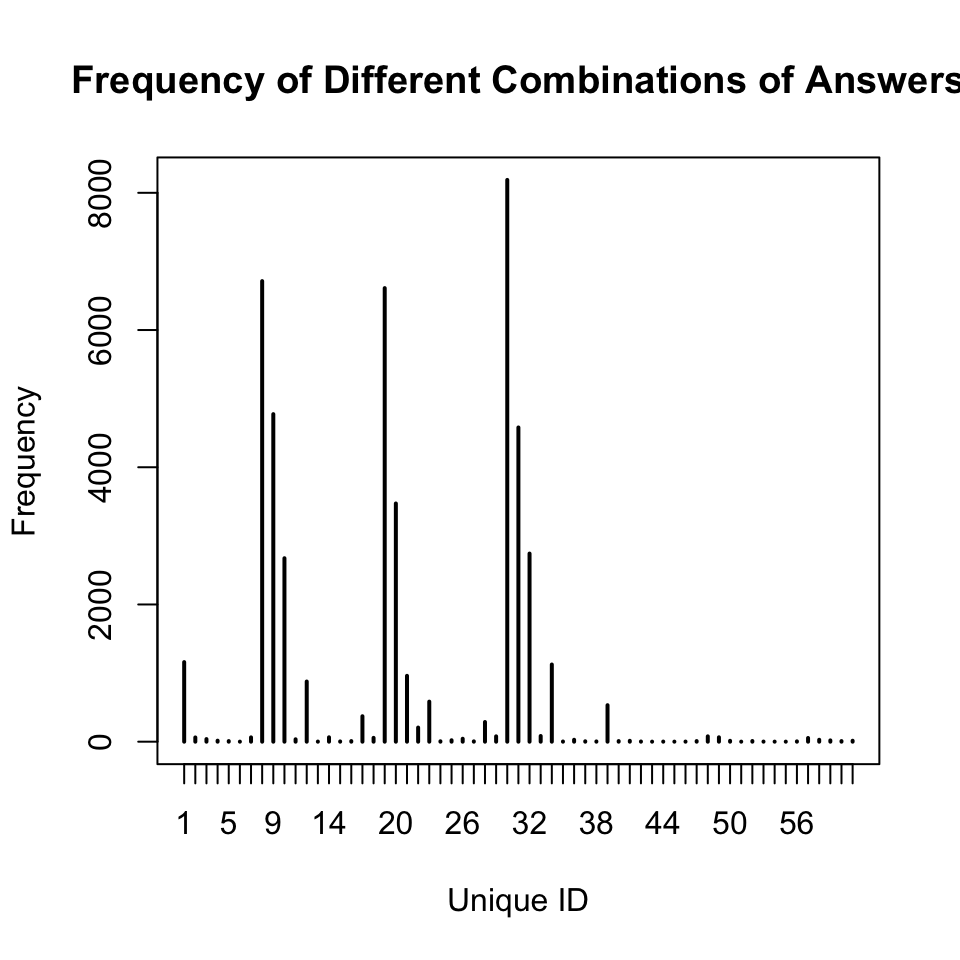
There are 6 unique combinations occueing more than 3000 times. When we investigate those:
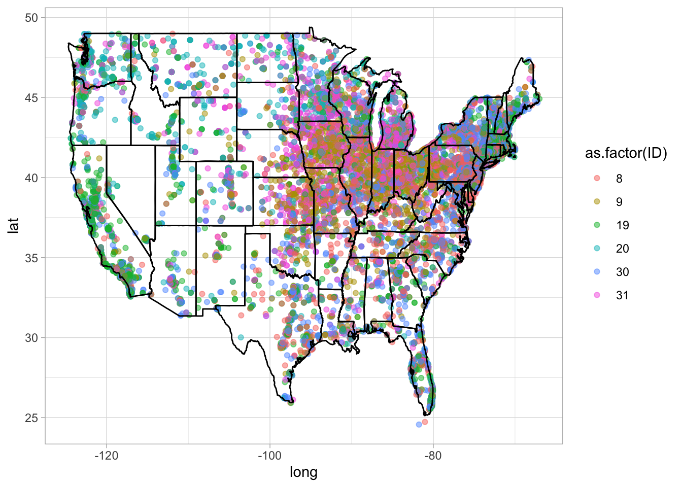
While combination 19 and 20 seem to dominate the west coast, the rest seem fairly evenly spread over the other regions (combination 9 and 8 seems promiment). There are precisely:
- Combination 19: Use ‘firefly’ and ‘soda’
- Combination 20: Use ‘firefly’ and ‘pop’
- Combination 9: Use ‘lightening bug’ and ‘pop’
- Combination 8: Use ‘lightening bug’ and pop’.
Dimension reduction methods
As a first step towards dimesnsion reduction, I used Principal Component Analysis. For this, I centered the data. If not, the geometric interpretation of PCA shows that the first principal component will be close to the vector of means and all subsequent PCs will be orthogonal to it, which will prevent them from approximating any PCs that happen to be close to that first vector. I didn’t however, scale the data, instead decided to scale it by the size of the zipcode.
A note:
It is not a good idea to perform PCA or any other metric-based dimensino reduction on the original data. The challenge with categorical variables is to find a suitable way to represent distances between variable categories and individuals in the factorial space. While PCA can be still be done for binary data, for categorical data,
Results of PCA
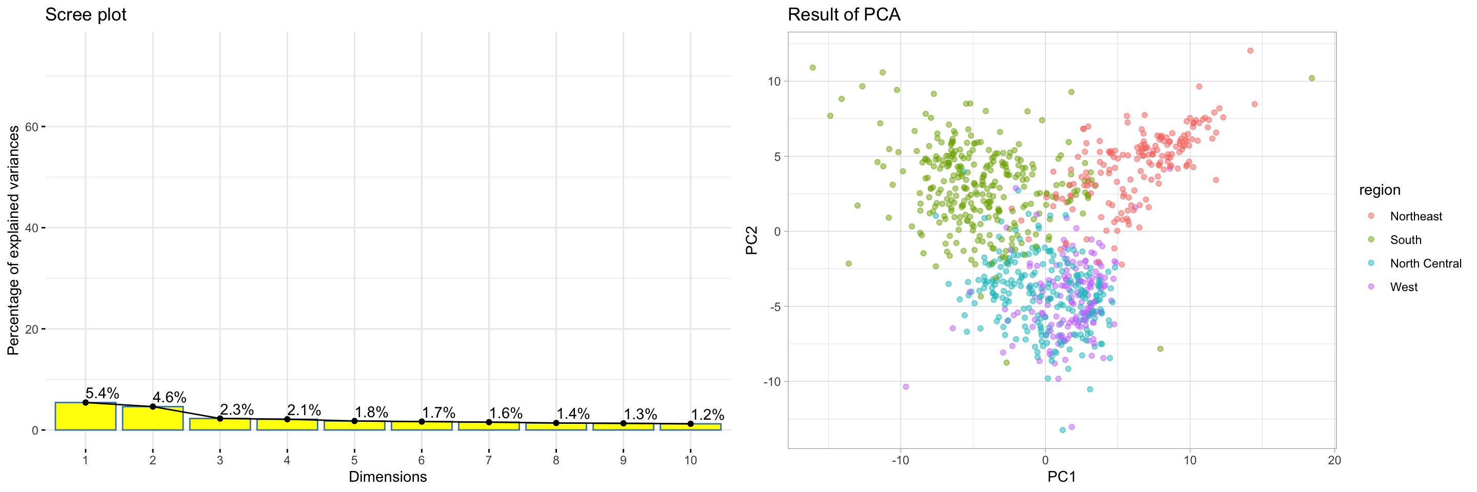
When I colour the observations by region, theres seem to some clusters, but because the Screeplot is not explaining a lot of variation in the first 10 dimesnions, I decide to conduct a TNSE and metric Multi Dimensional Scaling.
t-Distributed Stochastic Neighbor Embedding (t-SNE) is a non-linear technique for dimensionality reduction. t-Distributed stochastic neighbor embedding (t-SNE) minimizes the divergence between two distributions: a distribution that measures pairwise similarities of the input objects and a distribution that measures pairwise similarities of the corresponding low-dimensional points in the embedding. It is mainly a data exploration and visualization technique.
Multi Dimensional Scaling (MDS) depends on a distance metric. For this dataset I chose pearson correlation, since I’m more interested in the ‘profile’ of an observation. Multidimensional scaling (MDS) is an established statistical technique that has sometimes been used in language study (see Wheeler (2005)).
The results are as follows:
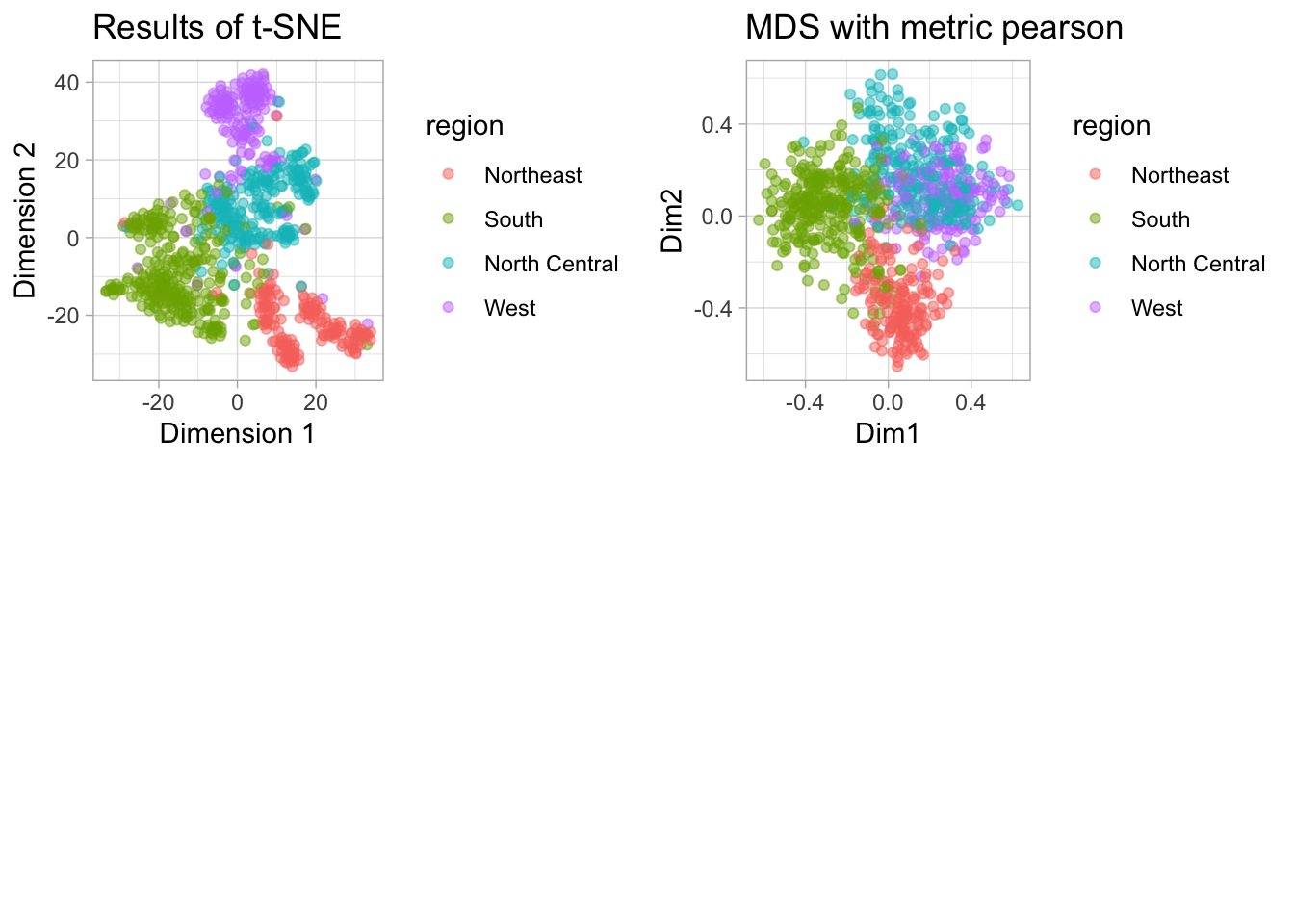
In tSNE and MDS we see that there seems to significant clustering according to region of the observation. t-SNE seems to clear the more clear and well-demarcated clusters. In PCA, however, clustering seems weaker.
Clustering
K- MEANS
My first approach was to use k-means to group the clusters. k-means is relatively computationally less expensive and is a good starting point to assess the validity of clusters. it’s useful when we have some sort of a plausible idea of how many clusters exist in the dataset.
I tried three metrics - Silhouette, Within sum of squares, and gap statistic to arrive at an optimal \(k\). ‘WSS’ is usually ambiguous and unreliable.
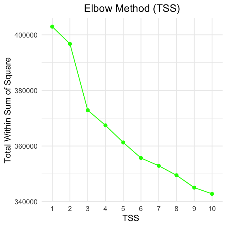
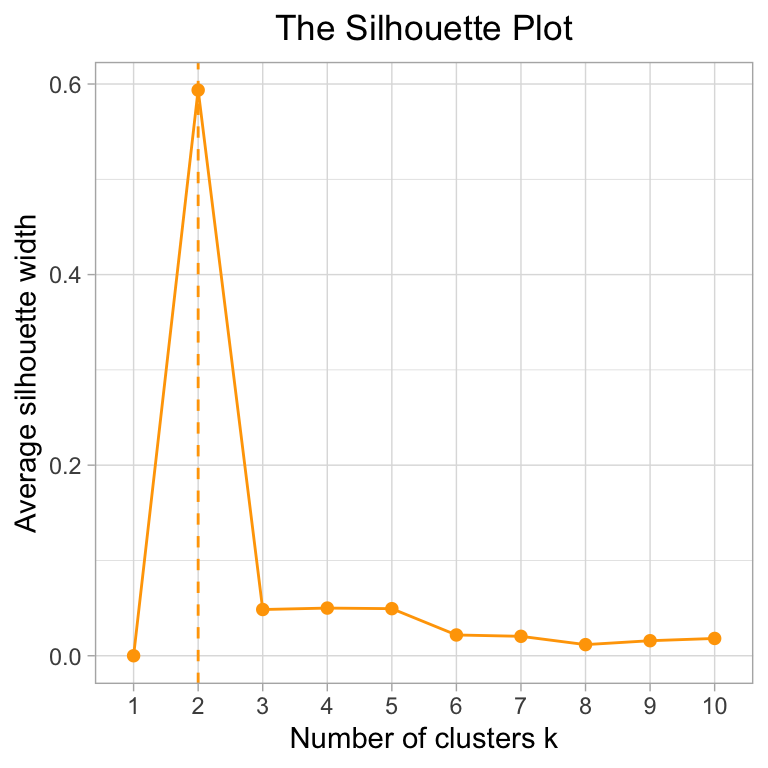
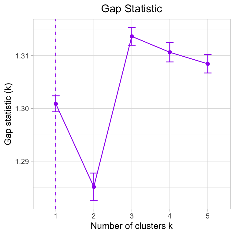
Both the Silhouette Method and Gap Statistic suggest less than 4 clusters. However, when we run a k-means with \(k\) = 2,3,4 and 5, we see that k = 4 seems to give the most uniform groups: (CROSSTALK WIDGET)
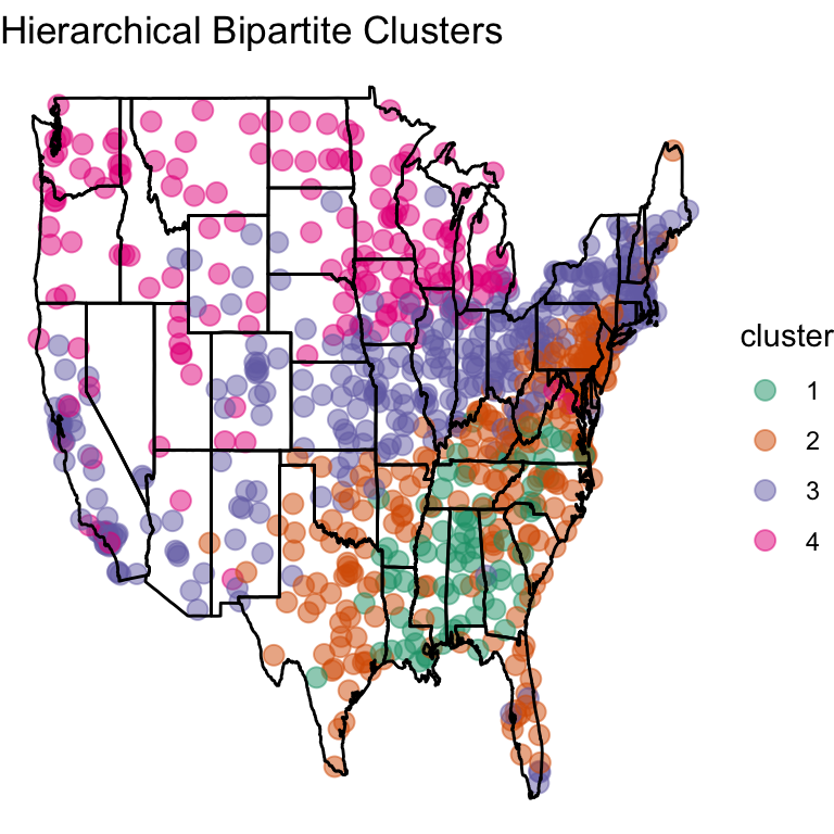
Hierarchical Bipartite Spectral Graph Partioning
The BiSGP method is based on calculating the singular value decomposition of the input matrix. The hierarchical clustering is obtained by repeatedly clustering the input matrix into two groups. An extensive mathematical explanation as well as an example of the BiSGP method is provided by Wieling and Nerbonne (2010, 2011). Dhillon first introduced this in his 2003 paper: https://www.cs.utexas.edu/users/inderjit/public_papers/kdd_bipartite.pdf
Importance Within A Cluster
Wieling and Nerbonne (2011) proposed a method to measure the importance of a linguistic feature (in our case a specific answer option) in a cluster by combining two measures, representativeness and distinctiveness.
Representativeness of a variant measures how frequently it occurs in the postcode areas in the cluster. For example, if a cluster consists of ten postcode areas and the variant occurs uniquely in six postcode areas, the representativeness is 0.6.
Distinctiveness of a variant measures how frequently the variant occurs within as opposed to outside the cluster (while taking the relative size of the clusters into account). For example, a distinctiveness of 1 indicates that the variant is not used outside of the cluster.
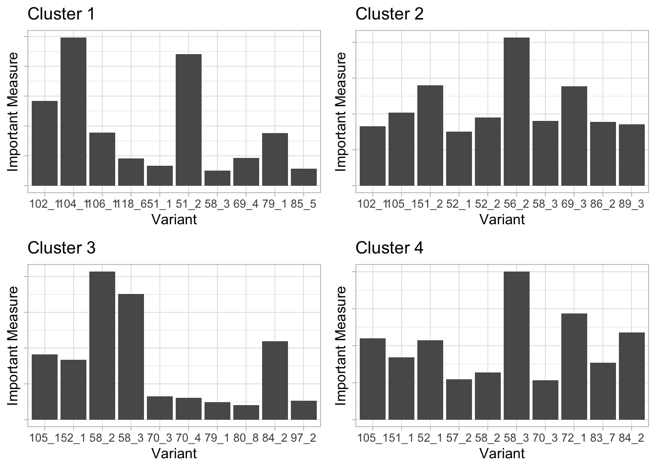
For example, we find that in Cluster 4, the two important questions variants are in Q58, same as Cluster 3. Taking a look at the questinos database tells us that this question is Which of these terms do you prefer for a sale of unwanted items on your porch, in your yard, etc.?
In cluster 2, one of the most important question is about correct use of Pantyhose are so expensive anymore that I just try to get a good suntan and forget about it.
Similarly in cluster 1 one of the most important questions is What do you call a public railway system (normally underground)? and *“Would you say ‘Are you coming with?’ as a full sentence, to mean ‘Are you coming with us?’*
.
Stability of findings to perturbation
Since k-means and BiSGP depend on random selection of center points, it influences the stability of conclusions. BiSGP method seemed pretty stable because it gave almost the same top 10 most relevant variants for each time I ran the code with different seeds.
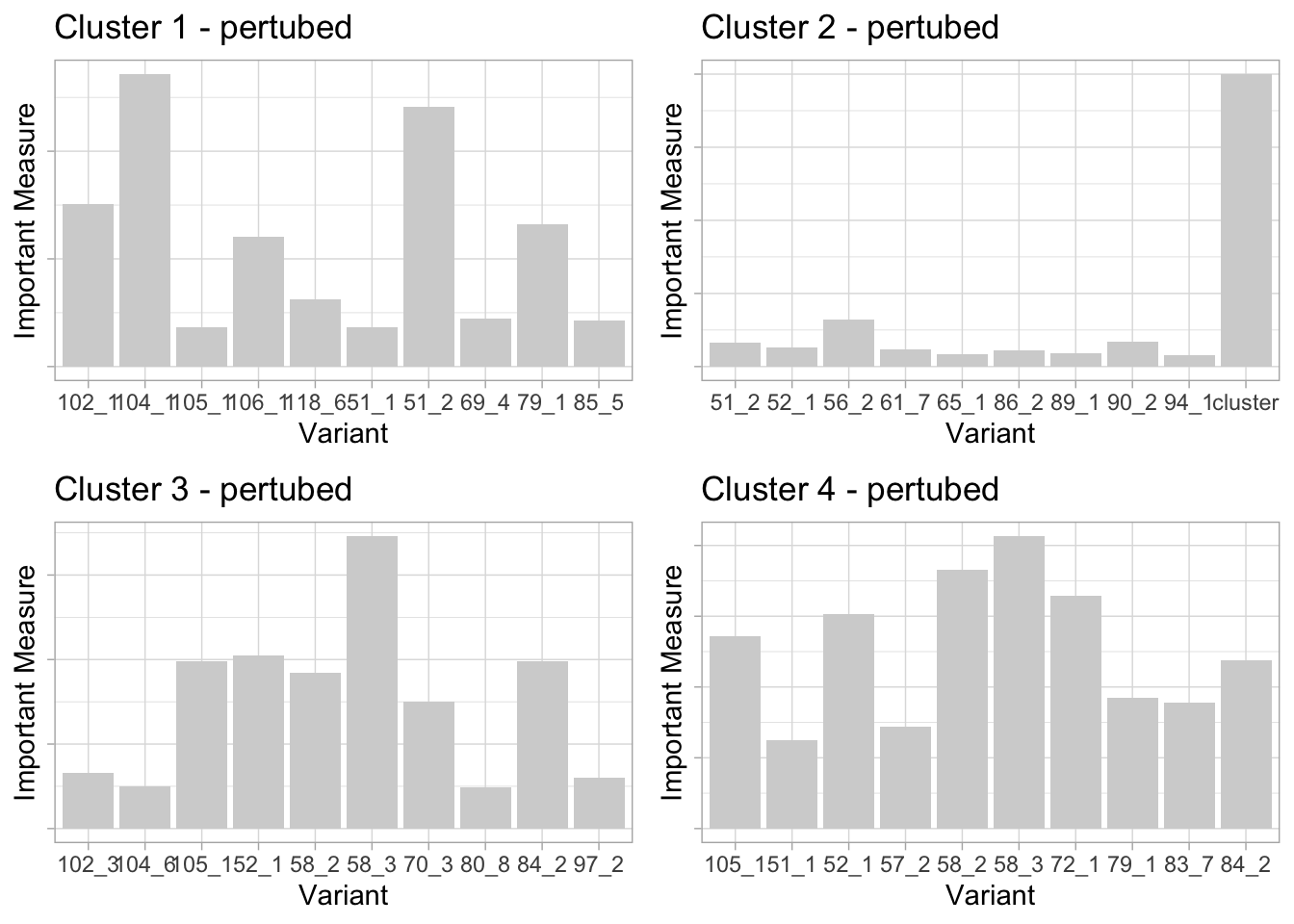
We see that the ‘most important’ questions do seem to change we subsample. I find to be logical because of the clustering is being done on the rows and the columns in BiSGP.
k-means
For k-means,I subsampled from the data 100 times, and averaged the ‘center matrix’ and compared it the center matrix to the original data.
The centers were off at an average of 3.6 units.
Conclusion
Reshaping data to make it suitable for analyses is very important. In a data structure like this, many important restructuring decisions, like whether to turn categorical to binary, to scale or not, which distance metric to use, all matter as much as the method of dimesion reduction/ clustering we attempt to do.
Dialectrometry and linguistic data in general has great scope for complex analyses, and can be used not only to ascertain spatial trends but perhaps also population characteristics like gender, age, etc.
References
Bipartite spectral graph partitioning for clustering dialect varieties and detecting their linguistic features - Martijn Weiling, John Nerbonne
Co-clustering documents and words using Bipartite Spectral Graph Partitioning - Inderjit S. Dhillon