Get your uber data
requesting data from uber
The purpose of this exercise is to visualise how I use my uber data. Uber records are pretty useful - just ask uber to email you your data: https://help.uber.com/driving-and-delivering/article/request-your-personal-uber-data?nodeId=fbf08e68-65ba-456b-9bc6-1369eb9d2c44
I'm removing remote 2020 and 2015 (it contains only one day) for now because it might skew the data.
reading in the data
myrides = read.csv("https://raw.githubusercontent.com/malvikarajeev/uberAnalysis/master/trips_data.csv")

head(myrides)
## City Product.Type Trip.or.Order.Status Request.Time
## 1 Los Angeles UberX COMPLETED 2020-02-17 04:43:38 +0000 UTC
## 2 Los Angeles UberX COMPLETED 2020-02-17 01:17:06 +0000 UTC
## 3 Los Angeles UberX COMPLETED 2020-02-16 20:29:34 +0000 UTC
## 4 Los Angeles UberX COMPLETED 2020-02-16 18:45:42 +0000 UTC
## 5 Los Angeles UberX COMPLETED 2020-02-16 00:17:16 +0000 UTC
## 6 Los Angeles UberX DRIVER_CANCELED 2020-02-15 23:36:22 +0000 UTC
## Begin.Trip.Time Begin.Trip.Lat Begin.Trip.Lng
## 1 2020-02-17 04:52:00 +0000 UTC 34.08361 -118.3521
## 2 2020-02-17 01:19:19 +0000 UTC 33.99775 -118.4748
## 3 2020-02-16 20:35:00 +0000 UTC 33.96174 -118.3673
## 4 2020-02-16 18:51:31 +0000 UTC 33.98221 -118.4594
## 5 2020-02-16 00:23:12 +0000 UTC 34.01283 -118.4966
## 6 1970-01-01 00:00:00 +0000 UTC 34.01028 -118.4934
## Begin.Trip.Address
## 1 7422 Melrose Ave, Los Angeles, CA 90046, US
## 2 423 Rose Ave, Venice, CA 90291, US
## 3 621 W Manchester Blvd, Inglewood, CA 90301, US
## 4 4100 Admiralty Way, Marina del Rey, CA 90292, US
## 5 111 Broadway, Santa Monica, CA 90401, US
## 6
## Dropoff.Time Dropoff.Lat Dropoff.Lng
## 1 2020-02-17 05:01:35 +0000 UTC 34.09819 -118.3077
## 2 2020-02-17 01:29:59 +0000 UTC 33.98216 -118.4595
## 3 2020-02-16 20:55:09 +0000 UTC 33.97935 -118.4664
## 4 2020-02-16 19:07:13 +0000 UTC 33.96225 -118.3671
## 5 2020-02-16 00:46:38 +0000 UTC 33.98220 -118.4595
## 6 1970-01-01 00:00:00 +0000 UTC 34.01351 -118.4972
## Dropoff.Address
## 1 5419 W Sunset Blvd, Los Angeles, CA 90027, US
## 2 4100 Admiralty Way, Marina del Rey, CA 90292, US
## 3 Venice Beach Pier Public Parkingl Lot, Unnamed Road, Marina Del Rey, CA 90292, United States
## 4 621 W Manchester Blvd, Inglewood, CA 90301, US
## 5 4100 Admiralty Way, Marina del Rey, CA 90292, US
## 6 4100 Admiralty Way, Marina del Rey, CA 90292, US
## Distance..miles. Fare.Amount Fare.Currency
## 1 3.56 9.14 USD
## 2 2.21 7.43 USD
## 3 7.27 11.65 USD
## 4 7.24 10.63 USD
## 5 3.81 10.30 USD
## 6 0.00 5.00 USDmyrides$completed = ifelse(myrides$Trip.or.Order.Status == 'COMPLETED', T, F)
##basic eda
myrides$time_started = as.POSIXct(strptime(myrides$Begin.Trip.Time, "%Y-%m-%d %H:%M:%S"))
myrides$year = year(myrides$time_started)
##remove 1970 and not completed
myrides = myrides %>% filter(!(year == 1970 | year == 2020 | year == 2015))
myrides = myrides %>% filter(Product.Type != 'UberEATS Marketplace')
myrides = myrides %>% filter(completed == T)
myrides$month_year = format(as.Date(myrides$Begin.Trip.Time), "%Y-%m")ggplot(myrides, aes(x = month_year)) +
geom_bar(aes(fill = as.factor(year))) +
scale_fill_brewer(palette="Set1") +
theme_tufte() +
theme(axis.text.x = element_blank()) +
labs(y = 'Frequency of Rides', x = 'Time Period') +
scale_fill_discrete(name = "Year")## Scale for 'fill' is already present. Adding another scale for 'fill', which
## will replace the existing scale.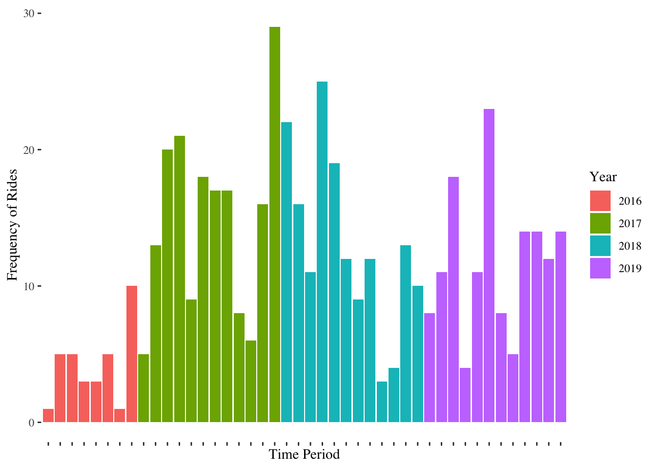
Seems like on an average I took about 10-20 rides a month, seemingly growing with every year. there seems to be a coherent pattern in that number of rides increase monotonically as we move from January to February (except for in 2018). The month of September-November seems generally low.
Now, I moved from New Delhi, India, to Berkeley, California, in the month of August, 2018. Can we see this move reflect different patterns?
average trip time.
myrides$time_ended = as.POSIXct(strptime(myrides$Dropoff.Time, "%Y-%m-%d %H:%M:%S"))
myrides$duration_mins = myrides$time_ended - myrides$time_started
myrides$duration_mins = as.integer(myrides$duration_mins)

ggplot(myrides, aes(y = duration_mins, x = month_year)) + geom_boxplot() +
  theme_tufte() +
  theme(axis.text.x = element_blank()) +
  labs(y = 'Distribution of Rides', x = 'Time Period') +
  scale_fill_discrete(name = "Year")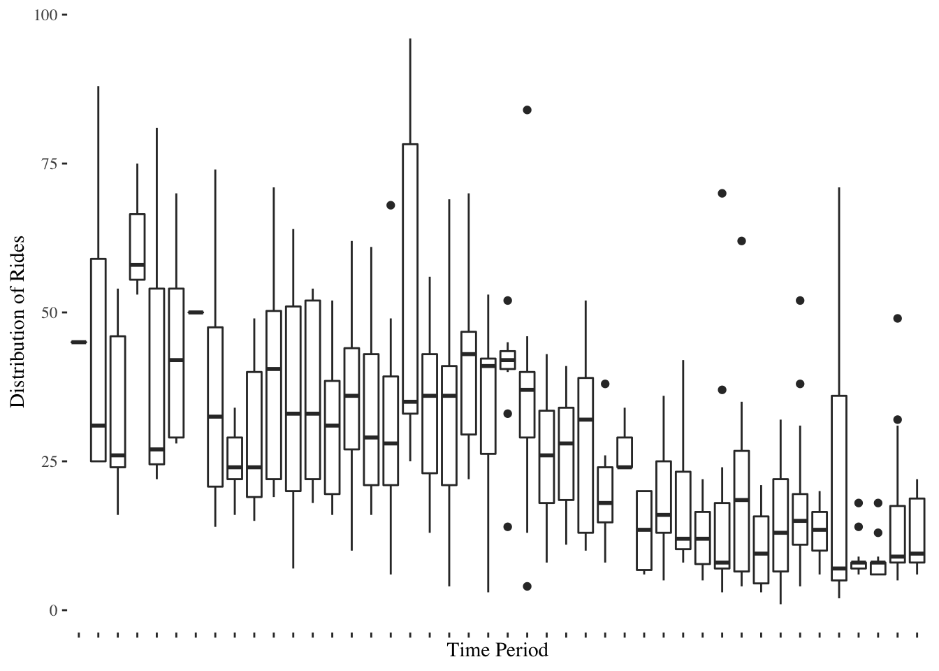
The average time of my rides is decreasing: perhaps it makes sense, the traffic in New Delhi is insane compared to the traffic in Berkeley.
fare habits
I wanted to group by year, and get the cumulative fare for each year by month. In the pursuit of this, I found a function called ave
fare_wise = function(currency){
  fares = myrides %>%
          filter(Fare.Currency == currency) %>%
          group_by(year, month_year) %>%
          summarise(monthly_fare = sum(Fare.Amount, na.rm = T))
  fares$cumulative_fare = ave(fares$monthly_fare, fares$year, FUN = cumsum)
  return(fares)
}

inr = fare_wise('INR')
## `summarise()` regrouping output by 'year' (override with `.groups` argument)##Adding year
##
ggplot(inr) +
geom_point(aes(y = cumulative_fare, x = month_year, color = factor(year))) +
theme_tufte() +
transition_states(year, wrap = T) 
  # labs(title = "Year: {frame_time}") +
  # view_follow(fixed_x = T)

# anim_save("inr.gif", animation = gg, path = "/figures")
What the hell was I doing in 2017... damn.
temp = myrides %>% filter(Begin.Trip.Lat * Begin.Trip.Lng != Dropoff.Lat*Dropoff.Lng) %>% filter(Fare.Currency == 'USD')


usa_map = map_data("county")

ca_df <- usa_map %>% filter(region == 'california')

# ggplot() +
#   geom_polygon(data = ca_df, aes(x=long, y = lat)) +
#   coord_fixed(1.3) +
#   geom_curve(data=temp,
#              aes(x=Begin.Trip.Lng, y=Begin.Trip.Lat, xend=Dropoff.Lng, yend=Dropoff.Lat),
#              col = "#b29e7d", size = 1, curvature = .2) +
#   geom_point(data=temp,
#              aes(x=Dropoff.Lng, y=Dropoff.Lat),
#              colour="blue",
#              size=1.5) +
#   geom_point(data=temp,
#              aes(x=Begin.Trip.Lng, y=Begin.Trip.Lat),
#              colour="blue") +
#   theme(axis.line=element_blank(),
#         axis.text.x=element_blank(),
#         axis.text.y=element_blank(),
#         axis.title.x=element_blank(),
#         axis.title.y=element_blank(),
#         axis.ticks=element_blank(),
#         plot.title=element_text(hjust=0.5, size=12))
library(shiny)
library(ggmap)
library(ggplot2)
ui <- fluidPage(
titlePanel("My Uber Rides"),
sidebarLayout(
# sidebarPanel(
# radioButtons("radio", label = h4("Choose currency"),
# choices = list("USD" = 'USD', "INR" = 'INR')),
# radioButtons("interval", label = h4("show time of day?"),
# choices = list("Yes" = TRUE, "No" = FALSE)),
selectInput("month_year", label = "Choose Month and Year",
choices = unique(temp$month_year)),
sliderInput("duration_ride", "Duration of Rides", min = 1, max = max(temp$duration), value = c(1,10))
),
mainPanel(plotOutput(outputId = "my_map")
)
)
)
#load()
server <- function(input, output) {
outputR = reactive({
req(input$duration_ride)
req(input$month_year)
temp2 = temp%>% filter(duration_mins <= input$duration_ride[2] & duration_mins >= input$duration_ride[1]) %>% filter(month_year == input$month_year)
usa_map = map_data("county")
ca_df <- usa_map %>% filter(region == 'california')
long = mean(temp2$Dropoff.Lng, na.rm = T)
latt = mean(temp2$Dropoff.Lat, na.rm = T)
g = ggmap(get_googlemap(c(long, latt),
zoom = 15 , scale = 2,
maptype ='roadmap',
color = 'color', archiving = T)) +
geom_segment(data=temp2,
aes(x=Begin.Trip.Lng, y=Begin.Trip.Lat, xend=Dropoff.Lng, yend=Dropoff.Lat),
col = "black", size = 0.3, arrow = arrow()) +
geom_point(data=temp2,
aes(x=Dropoff.Lng, y=Dropoff.Lat,
colour="red"),
alpha = 0.5) +
geom_point(data=temp2,
aes(x=Begin.Trip.Lng, y=Begin.Trip.Lat,
colour="blue"), alpha = 0.5) +
scale_color_identity(
breaks = c("red", "blue"),
labels = c("Drop off Point", "Pick up point"),
guide = "legend")
g
})
output$my_map= renderPlot({outputR()})
}
shinyApp(ui = ui, server = server)